library(dplyr)
library(ggplot2)
library(forcats)
library(knitr)
library(tidyverse)

ggplot(starwars, aes(y = hair_color)) +
  geom_bar()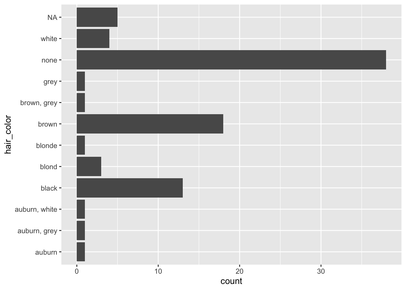
El objetivo del paquete forcats es proporcionar una serie de herramientas útiles que resuelven problemas comunes con los factores. Los factores son útiles cuando se tiene datos categóricos, variables que tienen un conjunto fijo y conocido de valores, y cuando se desea mostrar vectores de caracteres en un orden no alfabético.
library(dplyr)
library(ggplot2)
library(forcats)
library(knitr)
library(tidyverse)
ggplot(starwars, aes(y = hair_color)) +
geom_bar()
Este gráfico muestra los colores de cabello de los personajes de Star Wars, pero sería más útil si el gráfico estuviera ordenado por frecuencia. Para hacerlo, podemos usar la función fct_infreq():
ggplot(starwars, aes(y = fct_infreq(hair_color))) +
  geom_bar()
Existen dos formas de representar un valor faltante en un factor:
is.na() lo reporta como faltante.f <- factor(c("x", "y", NA))
levels(f)[1] "x" "y"is.na(f)[1] FALSE FALSE TRUEis.na() no lo reporta como faltante. Esto requiere un poco más de trabajo para crear, porque por defecto factor() usa exclude = NA.f <- factor(c("x", "y", NA), exclude = NULL)
levels(f)[1] "x" "y" NA is.na(f)[1] FALSE FALSE FALSEPara corregir el problema, podemos usar fct_na_value_to_level() para convertir el NA en el valor a un NA en los niveles:
ggplot(starwars, aes(y = fct_infreq(fct_na_value_to_level(hair_color)))) +
  geom_bar() +
  labs(y = "Color de Cabello")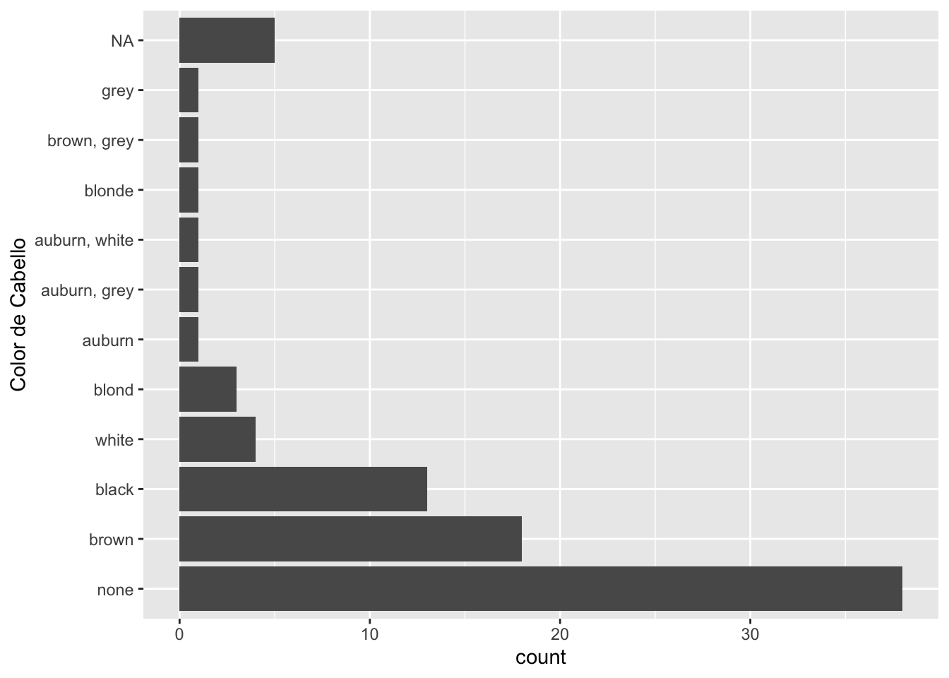
En caso de requerir la operación inversa, podemos usar fct_na_level_to_value().
Revisemos el color de piel de los personajes de Star Wars:
starwars |>
  count(skin_color, sort = TRUE)
# A tibble: 31 × 2
skin_color n
<chr> <int>
1 fair 17
2 light 11
3 dark 6
4 green 6
5 grey 6
6 pale 5
7 brown 4
8 blue 2
9 blue, grey 2
10 none 2
# ℹ 21 more rowsHagamos un gráfico de barras con los todos los colores de piel:
starwars |>
  count(skin_color, sort = TRUE) |>
  ggplot(aes(x = skin_color, y = n, fill = skin_color)) +
  geom_col()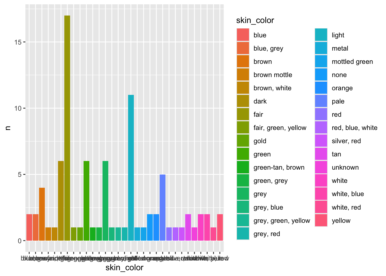
Si observamos los colores de piel, podríamos querer reducir los niveles a solo los cinco más comunes:
starwars |>
  mutate(skin_color = fct_lump(skin_color, n = 5)) |>
  count(skin_color, sort = TRUE)
# A tibble: 6 × 2
skin_color n
<fct> <int>
1 Other 41
2 fair 17
3 light 11
4 dark 6
5 green 6
6 grey 6Podemos usar prop para agrupar los niveles en función de la proporción de observaciones:
starwars |>
  mutate(skin_color = fct_lump(skin_color, prop = .1)) |>
  count(skin_color, sort = TRUE)
# A tibble: 3 × 2
skin_color n
<fct> <int>
1 Other 59
2 fair 17
3 light 11Esta función es útil cuando se quiere aplicar junto con otras funciones de dplyr. Por ejemplo, podemos calcular la masa promedio de los personajes de Star Wars por color de ojos. Eso si solo queremos los seis colores de ojos más comunes.
avg_mass_eye_color <- starwars |>
  mutate(eye_color = fct_lump(eye_color, n = 6)) |>
  group_by(eye_color) |>
  summarise(mean_mass = mean(mass, na.rm = TRUE))

kable(avg_mass_eye_color)| eye_color | mean_mass |
|---|---|
| black | 76.28571 |
| blue | 86.51667 |
| brown | 66.09231 |
| orange | 282.33333 |
| red | 81.40000 |
| yellow | 81.11111 |
| Other | 68.42857 |
Otra forma de hacer esto es con fct_other():
starwars |>
  mutate(skin_color = fct_other(skin_color,
    keep = c("fair", "dark", "green", "light")
  )) |>
  pull(skin_color)
[1] fair Other Other Other light light light Other light fair fair fair
[13] Other fair green Other fair fair green Other fair Other green dark
[25] light Other fair fair Other Other fair Other fair light Other Other
[37] green fair Other Other dark fair Other Other Other Other Other Other
[49] Other dark Other green Other dark Other Other Other Other dark light
[61] fair green Other Other light fair Other Other Other Other Other Other
[73] fair Other Other Other Other Other Other light Other Other dark light
[85] light Other Other
Levels: dark fair green light Otherstarwars |>
mutate(skin_color = fct_collapse(skin_color,
"green" = c("green", "green-tan, brown", "mottled green")
)) |>
pull(skin_color) [1] fair gold white, blue
[4] white light light
[7] light white, red light
[10] fair fair fair
[13] unknown fair green
[16] green fair fair
[19] green pale fair
[22] metal green dark
[25] light brown mottle fair
[28] fair brown grey
[31] fair green fair
[34] light orange grey
[37] green fair blue, grey
[40] grey, red dark fair
[43] red pale blue
[46] grey, blue blue, grey white, blue
[49] grey, green, yellow dark pale
[52] green brown dark
[55] pale white orange
[58] blue dark light
[61] fair green yellow
[64] yellow light fair
[67] tan tan fair, green, yellow
[70] brown grey grey
[73] fair silver, red green, grey
[76] grey red, blue, white brown, white
[79] brown light pale
[82] grey dark light
[85] light none none
29 Levels: blue blue, grey brown brown mottle brown, white dark ... yellowstarwars |>
mutate(
skin_color = factor(skin_color),
skin_color = fct_collapse(
skin_color,
"multicolor" = levels(skin_color)[str_detect(levels(skin_color), ",\\s")],
"green" = levels(skin_color)[str_detect(levels(skin_color), "green")],
"brown" = levels(skin_color)[str_detect(levels(skin_color), "brown")],
"blue" = levels(skin_color)[str_detect(levels(skin_color), "blue")],
)
) |>
pull(skin_color) [1] fair gold blue white light light
[7] light multicolor light fair fair fair
[13] unknown fair green brown fair fair
[19] green pale fair metal green dark
[25] light brown fair fair brown grey
[31] fair green fair light orange grey
[37] green fair blue multicolor dark fair
[43] red pale blue blue blue blue
[49] green dark pale green brown dark
[55] pale white orange blue dark light
[61] fair green yellow yellow light fair
[67] tan tan green brown grey grey
[73] fair multicolor green grey blue brown
[79] brown light pale grey dark light
[85] light none none
18 Levels: blue brown dark fair green gold grey multicolor light metal ... yellowlevels(factor(starwars$skin_color)) [1] "blue" "blue, grey" "brown"
[4] "brown mottle" "brown, white" "dark"
[7] "fair" "fair, green, yellow" "gold"
[10] "green" "green-tan, brown" "green, grey"
[13] "grey" "grey, blue" "grey, green, yellow"
[16] "grey, red" "light" "metal"
[19] "mottled green" "none" "orange"
[22] "pale" "red" "red, blue, white"
[25] "silver, red" "tan" "unknown"
[28] "white" "white, blue" "white, red"
[31] "yellow" Podemos usar fct_reorder() para reordenar una variable por otra, como ordenar por masa promedio:
avg_mass_eye_color |>
  pull(eye_color)
[1] black blue brown orange red yellow Other
Levels: black blue brown orange red yellow Otheravg_mass_eye_color |>
ggplot(aes(x = eye_color, y = mean_mass)) +
geom_col()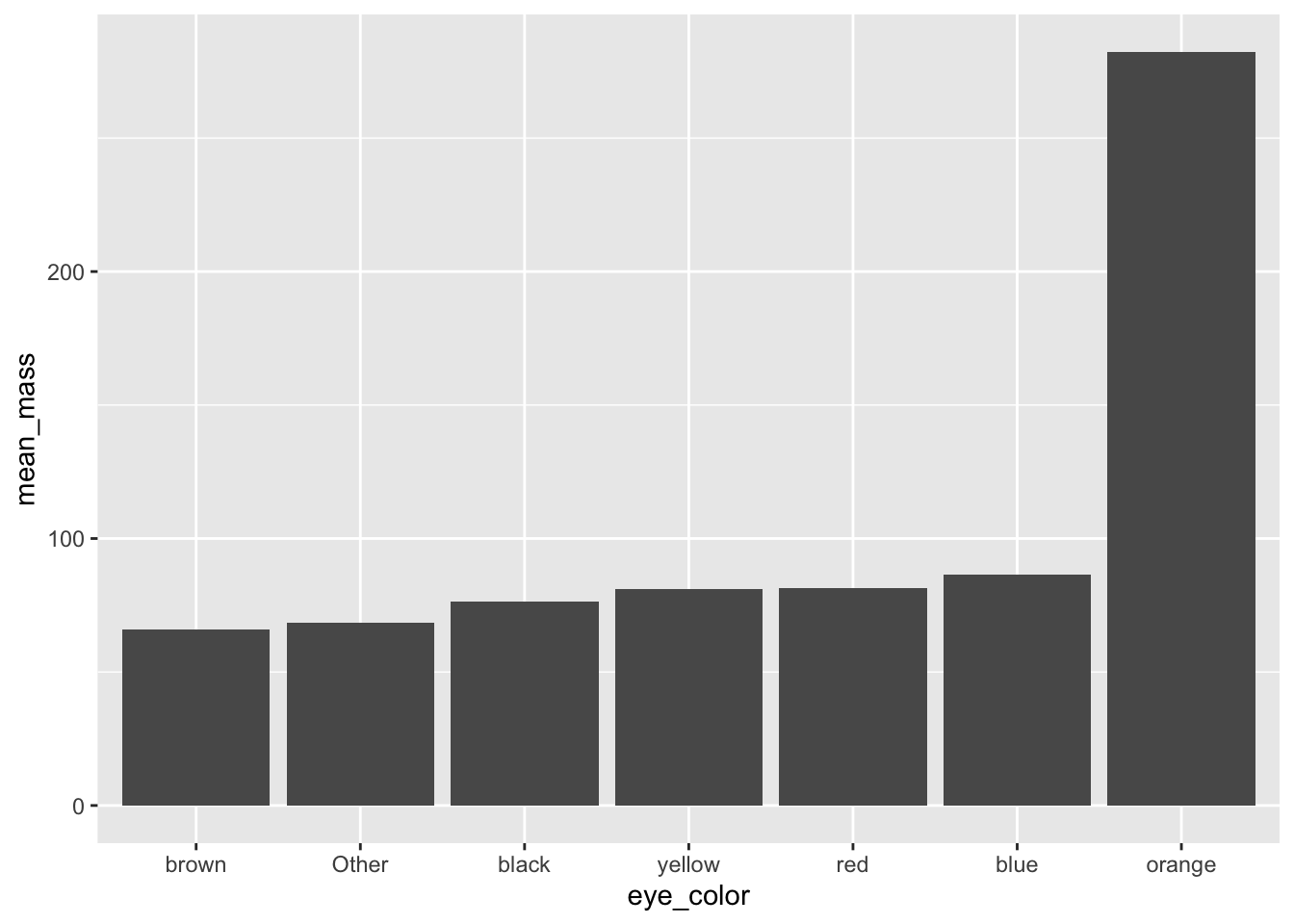
avg_mass_eye_color |>
  mutate(eye_color = fct_reorder(eye_color, mean_mass)) |>
  pull(eye_color)
[1] black blue brown orange red yellow Other
Levels: brown Other black yellow red blue orangeavg_mass_eye_color |>
mutate(eye_color = fct_reorder(eye_color, mean_mass)) |>
ggplot(aes(x = eye_color, y = mean_mass)) +
geom_col()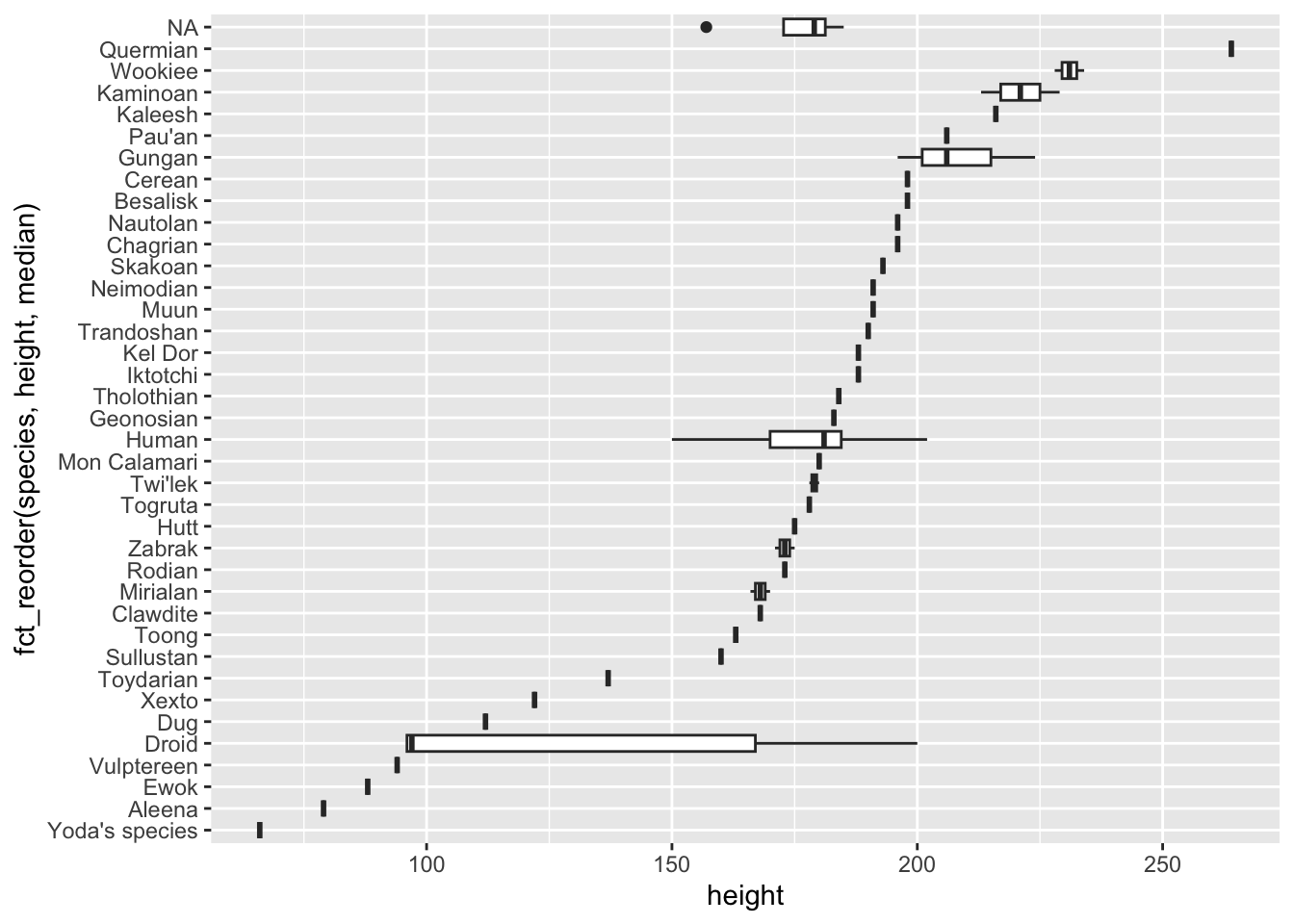
Otro ejemplo concreto
ggplot(starwars, aes(x = species, y = height)) +
  geom_boxplot() +
  coord_flip()
Warning: Removed 6 rows containing non-finite outside the scale range
(`stat_boxplot()`).
ggplot(starwars, aes(
  x = fct_reorder(species, height, median),
  y = height
)) +
  geom_boxplot() +
  coord_flip()
Warning: `fct_reorder()` removing 6 missing values.
ℹ Use `.na_rm = TRUE` to silence this message.
ℹ Use `.na_rm = FALSE` to preserve NAs.Warning: Removed 6 rows containing non-finite outside the scale range
(`stat_boxplot()`).
ggplot(starwars, aes(
  x = fct_reorder(species, height, median, .desc = TRUE),
  y = height
)) +
  geom_boxplot() +
  coord_flip()
Warning: `fct_reorder()` removing 6 missing values.
ℹ Use `.na_rm = TRUE` to silence this message.
ℹ Use `.na_rm = FALSE` to preserve NAs.Warning: Removed 6 rows containing non-finite outside the scale range
(`stat_boxplot()`).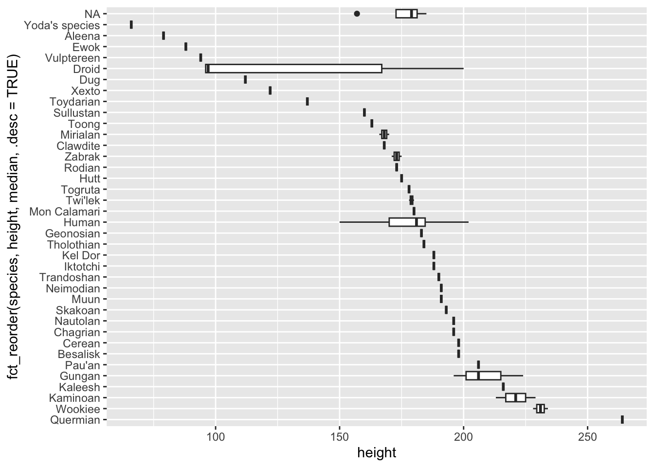
Podemos usar fct_relevel() cuando necesitamos reordenar manualmente los niveles de un factor:
reshuffled_income <- gss_cat$rincome |>
  fct_shuffle()

fct_relevel(reshuffled_income, c("Lt $1000", "$1000 to 2999")) |>
  levels()
[1] "Lt $1000" "$1000 to 2999" "Refused" "$8000 to 9999"
[5] "$6000 to 6999" "Don't know" "$7000 to 7999" "$10000 - 14999"
[9] "$5000 to 5999" "$4000 to 4999" "Not applicable" "No answer"
[13] "$25000 or more" "$20000 - 24999" "$15000 - 19999" "$3000 to 3999"